Mapping Airbnb listings, part 1
Intro
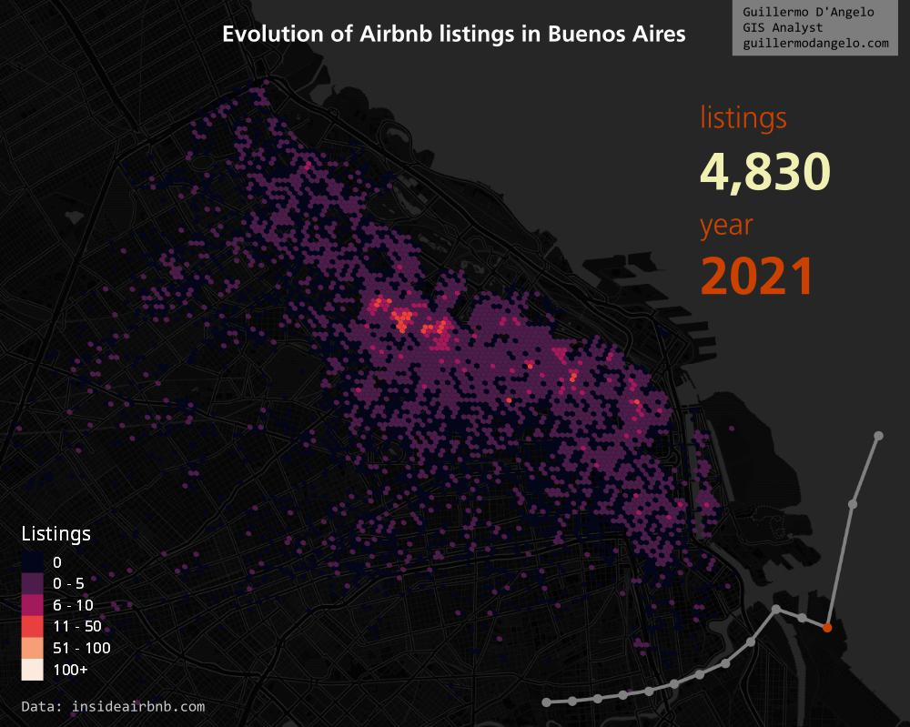
This post appeared recently on my LinkedIn feed. The author kindly pointed me to the source of the data, which is this awesome project called Inside Airbnb
I decided to make something similar, but less stylized.
In this tutorial, I share how I did it, so you can play around with the data and make your own maps, using the data from Inside Airbnb. The tutorial is divided in two parts, first the data processing and then the cartography. You may need to have some basic Python knowledge to follow the process.
Data processing
The processing was done using Python, so you must have a Python environment with pandas, numpy, matplotlib, h3pandas and jupyter installed.
I'll post each code block of the original Jupyter Notebook, which you can access by clicking in this link
First, chose the city you want to map and download the data. You have plenty of options. We only need the listings.csv.gz and reviews.csv files.
Load the packages and set the input and output paths. We also set the scale of the H3 grid, which in this case will be 10.
import pandas as pd
import numpy as np
import matplotlib.pyplot as plt
import h3pandas as h3pd

listings_file = 'buenos_aires.csv.gz'
reviews_file = 'reviews_buenos_aires.csv'
output_file = 'buenos_aires_hex_listings.gpkg'
hex_scale = 10
Load listing and reviews, and generate a variable to identify the year of every review.
# load listings
listings = pd.read_csv(listings_file, usecols=['id', 'latitude', 'longitude'])
listings.rename(columns={'latitude': 'lat', 'longitude': 'lng'}, inplace=True)

# load reviews
rev = pd.read_csv(reviews_file)
rev['year'] = pd.to_datetime(rev.date).dt.year
rev['year'] = 'reviews_' + rev['year'].astype(str)

cols = list(rev.year.unique())
cols.sort()
Then, in order to find if every listing has reviews for every year between 2010 and 2023, we make a cross tabulation. We consider that a property that has at least one review was listed that year. Pandas crosstab will be the used function.
# crosstab
rev_crosstab = pd.crosstab(rev.listing_id, rev.year).reset_index()
print(rev_crosstab.shape)

# if there are reviews, we input True, else False
for col in cols:
    rev_crosstab[col] = np.where(rev_crosstab[col] >= 1, True, False)

rev_crosstab.head()
Let's make a bar plot to get a first glimpse of hour data, grouping by year.
# grouping by year
listings_acc = [sum(rev_crosstab[col]) for col in cols]
years = list(range(2010, 2024))

plt.bar(years, listings_acc, color='seagreen')
plt.title('Airbnb listings by year in Buenos Aires, Argentina')

# Add data labels above each bar
for year, nlistings in zip(years, listings_acc):
    plt.text(year, nlistings + 50, str(nlistings), ha='center', va='bottom', size=7)

# Remove all borders (top, right, left, bottom)
def remove_spines():
    ax = plt.gca()
    ax.spines['top'].set_visible(False)
    ax.spines['right'].set_visible(False)
    ax.spines['left'].set_visible(False)
    ax.spines['bottom'].set_visible(False)

remove_spines()

# Remove left ticks and tick labels
ax = plt.gca()
ax.tick_params(axis='y', left=False, labelleft=False)
plt.tick_params(axis='x', bottom=False)
plt.xticks(years, rotation=45)

plt.show()
Then we'll make a series of charts, one by year, that we'll later be using in our maps (this will be the matter of part 2). You'll have to change the values if you choose other city than Buenos Aires.
plt.ioff()

for year in years:
    plt.figure(figsize=(8, 6))  # Optional: Adjust the figure size if needed
    plt.plot(years, listings_acc,  linestyle='-', linewidth=4, color='grey')

    # Create the line plot and loop through the data points
    for i in range(len(years)):
        if years[i] == year:
            # Use a different color for the specific year (e.g., red)
            color = '#cb4200'
            plt.plot(years[i], listings_acc[i], marker='o', markersize=10, linestyle='-', color=color)
            if years[i] == 2020:
                plt.text(year, listings_acc[i] - 1500, str('COVID'), ha='center', va='bottom', size=14, color=color)
        else:
            # Use the default color for other years (e.g., blue)
            plt.plot(years[i], listings_acc[i], marker='o', markersize=10, linestyle='-', color='grey')

    # Optional: Customize the appearance (e.g., grid, axis limits)
    plt.xlim(min(years)-1, max(years)+1)
    plt.ylim(min(listings_acc)-600, max(listings_acc)+600)
    ax = plt.gca()

    ax.get_xaxis().set_visible(False)
    ax.get_yaxis().set_visible(False)

    remove_spines()

    plt.savefig(f'charts/listings_bsas_{year}.png', transparent=True)
Now we need to aggregate the data to our hex bins or H3 grid hexagons. Here we rely on a package called h3pandas, that will allow us to determine the hexagon for every lat/lon of the dataframe and then group the data easily.
merge = listings.merge(rev_crosstab, left_on='id', right_on='listing_id', how='inner')
hex = merge.h3.geo_to_h3(hex_scale)
hex.head(2)
Once we added the H3 id to our dataframe, we need to aggregate it, counting the listings for every year and every hexagon. We use the "h3_to_geo_boundary" method to generate a polygon.
def agg_hex_processing(df, column, scale):
    '''Process a grouped hex grid'''
    hex_scale = 'h3_' + str(scale).zfill(2)
    hex_group = df.loc[:, column].to_frame().groupby(hex_scale)\
        .sum().h3.h3_to_geo_boundary()
    hex_group.rename({column: 'reviews'}, axis=1, inplace=True)
    hex_group['year'] = int(column.replace('reviews_', ''))

    return hex_group

review_cols = [f'reviews_{year}' for year in years]
all_hex = [agg_hex_processing(hex, col, hex_scale) for col in review_cols]
Finally, we need to concatenate all of our GeoPandas' GeoDataFrames into a new one, setting its CRS to EPSG:3857 (this is one of many you could use), and then exporting this dataframe to a file, in this case a GeoPackage. This file can be dragged and dropped to QGIS for further visualization.
# exports
all_hex_concat = pd.concat(all_hex).to_crs(3857)
all_hex_concat.to_file(output_file, driver='GPKG')
And that's it! We'll later be working with QGIS to make the maps we need.